What is a DataFrame?
A DataFrame is like a table structure with rows and columns because when we work with data in Python, we need a structure to store and organize it. That is the reason we have used a DataFrame.
You know that Excel has 1st, 2nd, 3rd rows and columns like Name, Age, Salary, and more. But a DataFrame is much more powerful because you can filter, clean, analyze, and visualize data with just a few lines of code.
Key Features of a DataFrame:
1) Labelled axes: This means that every row and column in a DataFrame has a label.
- Columns have names like “Age”, “Salary”, and more.
- Rows have an index (0, 1, 2 … by default, or custom labels.
This makes selecting data much easier than in plain lists or arrays. For example:
import pandas as pd

data = {'Name': ['Alice', 'Bob'], 'Age': [25, 30]}
df = pd.DataFrame(data, index=['a', 'b'])  # custom row labels

print(df)
print("Access Bob’s age:", df.loc['b', 'Age'])

// You don't have to remember positions, Just use tables.
2) Multiple data types: A single DataFrame can store different kinds of data in different columns, such as integers, floats, strings, and even other data types like dates.
For example:
data = {
    'Name': ['Alice', 'Bob'],
    'Age': [25, 30],
    'JoinDate': pd.to_datetime(['2024-01-01', '2024-02-15'])
}
df = pd.DataFrame(data)
print(df.dtypes)
- NumPy array holds the same type, but a DataFrame is flexible, just like an Excel, where one column is “Text” and another is “Numbers”.
3) Indexing and Selection: DataFrames support various ways to access and modify data, such as by column name, row index, or conditions. It means we can grab exactly the piece of data we need.
Example:
# Select a column
print(df['Age'])

# Select a row
print(df.loc[0])  # row by label/index

# Conditional selection
print(df[df['Age'] > 26])  # only people older than 26
- This is more powerful than plain lists.
4) In-built Data Operations: DataFrames have built-in functions for data cleaning, filtering, grouping, merging, and aggregation.
For example:
data = {
    'Name': ['Alice', 'Bob', 'Charlie', 'Alice'],
    'Sales': [200, 300, 150, 250]
}
df = pd.DataFrame(data)

# Group by Name and calculate total sales
print(df.groupby('Name')['Sales'].sum())

# Remove duplicates
print(df.drop_duplicates())
How To Create a DataFrame?
DataFrames can be created in multiple ways, such as from dictionaries, lists, or reading from a file (like a CSV file). Here are a few examples of creating DataFrames:
Example 1: Creating a DataFrame from a Dictionary
import pandas as pd

# Step 1: Make a dictionary (like a mini dataset of students)
student_data = {
    "Student": ["Aarav", "Sophia", "Liam"],
    "Marks": [88, 92, 79],
    "Country": ["India", "USA", "Canada"]
}

# Step 2: Convert dictionary to DataFrame
df = pd.DataFrame(student_data)

# Step 3: Print the DataFrame
print("Student Records:")
print(df)
Output:

Example 2: Creating a DataFrame from a CSV File
DataFrames can be easily created from external data sources like CSV files, which are common in data science projects.
Imagine you already have a .csv file that stores sales information. Instead of typing all the data manually, you can load it directly into a DataFrame.
import pandas as pd

# Step 1: Read data from a CSV file (assume the file exists in the same folder)
sales_df = pd.read_csv("sales_data.csv")

# Step 2: Show the first few rows to quickly check the data
print("First 5 rows of Sales Data:")
print(sales_df.head())
Your Possible CSV Content Look Like (sales_data.csv)
Product,Price,Units_Sold
Laptop,800,15
Phone,500,30
Tablet,300,20
Headphones,100,50
Output:

How To Access Data in a DataFrame?
Once we have created a DataFrame in Pandas, the next big step is retrieving the right data.
Imagine it like opening a spreadsheet, but we don’t need to open a full table, just want to a specific column, a row, or a slice of data. Pandas make this very flexible.
1) Accessing Columns
A column in a DataFrame is like a vertical slice of data. We can grab one or more columns using either bracket notation or dot notation.
For example:
import pandas as pd

# Sample DataFrame
data = {
    "Student": ["Aarav", "Sophia", "Liam"],
    "Marks": [88, 92, 79],
    "Country": ["India", "USA", "Canada"]
}
df = pd.DataFrame(data)

# Access a single column
print("Student Names:")
print(df["Student"])

# Access multiple columns
print("\n Student Names and Marks:")
print(df[["Student", "Marks"]])
Output of this code:

- Notice how selecting one column gives us a Series like a 1D list, while selecting multiple columns gives us another DataFrame.
2) Accessing Rows
Rows are horizontal records. We usually use .loc[] (label-based) or .iloc[] (index-based) to access them.
Example: Using .loc[]
- We use the row label like row number if not customized.
# Access the first row (label 0)
print("First Student Record:")
print(df.loc[0])
Output:

Example: Using .iloc[]
- .iloc[] is position-based indexing (like Python lists, starting from 0).
# Access rows at position 1 and 2
print("Student Records at Index 1 and 2:")
print(df.iloc[1:3])
Output:

Mixing Columns and Rows
- Sometimes we want a specific row + specific columns. Pandas allows us to combine both.
# Get Marks of the student at index 2
print("Marks of student at index 2:")
print(df.loc[2, "Marks"])
Output:

Data Manipulation with DataFrames
DataFrames provide numerous functions for data manipulation, which are essential for cleaning and preparing data before analysis.
How To Adding and Removing Columns?
Adding new columns or deleting existing ones is simple with DataFrames.
import pandas as pd

# Initial dataset
data = {
    'Name': ['Alice', 'Bob', 'Charlie'],
    'Age': [24, 27, 22],
    'City': ['New York', 'Paris', 'London']
}

df = pd.DataFrame(data)

# Adding a new column 'Country'
df['Country'] = ['USA', 'France', 'UK']

print("DataFrame after adding a column:")
print(df)

# Removing the 'Age' column
df.drop(columns=['Age'], inplace=True)

print("\nDataFrame after dropping 'Age' column:")
print(df)
Output:
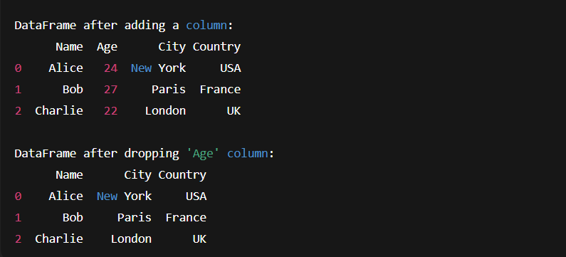
- In this code, we created a new column Country by simply assigning a list, and removed the Age column using .drop().
- This method is the same as adding and removing columns in Excel manually, but here, it takes just one line of Python.
How To Filtering Data?
DataFrames allow filtering data based on specific conditions, making it easy to work with only relevant data.
data = {
    'Name': ['Alice', 'Bob', 'Charlie', 'David'],
    'Age': [24, 27, 22, 30],
    'City': ['New York', 'Paris', 'London', 'Berlin']
}

df = pd.DataFrame(data)

# Filtering rows where Age > 23
filtered_df = df[df['Age'] > 23]

print("Filtered DataFrame (Age > 23):")
print(filtered_df)
Output:

3) Grouping and Aggregation
We use this method when we want to find some average grouping data.
data = {
    'Name': ['Alice', 'Bob', 'Charlie', 'David', 'Eva'],
    'Age': [24, 27, 22, 30, 29],
    'City': ['New York', 'Paris', 'London', 'Paris', 'London']
}

df = pd.DataFrame(data)

# Grouping by City and finding average Age
grouped_df = df.groupby('City')['Age'].mean()

print("Average Age by City:")
print(grouped_df)
Output:

- Here, Pandas grouped people based on their City and then calculated the mean Age for each group.
Data Analysis with Pandas DataFrames
DataFrames provide built-in functions to quickly analyze and describe data, allowing data scientists to gain insights with minimal code.
Descriptive Statistics
The describe( ) method provides a quick statistical summary of numerical columns, including mean, median, standard deviation, and more.
This method is like asking Pandas, “Tell me the overall picture of my dataset.”
import pandas as pd

# Sample dataset
data = {
    'Product': ['A', 'B', 'C', 'D'],
    'Price': [100, 200, 300, 400],
    'Units_Sold': [50, None, 40, 70]
}

df = pd.DataFrame(data)

# Summary statistics
print("Summary Statistics:")
print(df.describe())
Output:
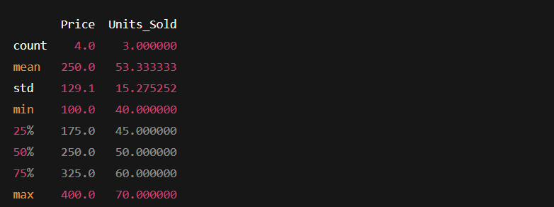
- We immediately know all prices and units of data without calculating them manually.
Handling Missing Values
In real-world data, missing values are very common, like someone not filling in a survey question. Pandas gives us two main choices:
- Fill Missing Values
- Drop Missing Values
(a) Fill Missing Values
df['Units_Sold'].fillna(0, inplace=True)
print(df)
- this replaces missing values with 0. You can replace with mean, median, or custom values depending on context.
(b) Drop Missing Values
df.dropna(inplace=True)
print(df)
- This removes any row that has missing data.
Merging and Joining DataFrames
Our data is split across multiple tables, and Pandas allows you to combine them using the SQL joins method.
Example of Merging DataFrames
data1 = {'ID': [1, 2, 3], 'Name': ['Alice', 'Bob', 'Charlie']}
data2 = {'ID': [1, 2, 4], 'Score': [85, 90, 78]}

df1 = pd.DataFrame(data1)
df2 = pd.DataFrame(data2)

# Merging DataFrames on 'ID' column
merged_df = pd.merge(df1, df2, on='ID', how='inner')
print(merged_df)
Output:

Example: Simple Data Analysis with a DataFrame
Here’s a complete example of loading, cleaning, and analyzing data in a DataFrame.
import pandas as pd

# Step 1: Create a DataFrame (sample shop data)
data = {
    'Item': ['Laptop', 'Phone', 'Tablet', 'Headphones'],
    'Price': [800, 500, 300, 100],
    'Quantity_Sold': [10, None, 25, 60]
}
df = pd.DataFrame(data)

# Step 2: Handle missing values (replace with median instead of mean)
df['Quantity_Sold'].fillna(df['Quantity_Sold'].median(), inplace=True)

# Step 3: Add a new column for total sales
df['Sales'] = df['Price'] * df['Quantity_Sold']

# Step 4: Show the updated table
print("Sales Data Table:")
print(df)

# Step 5: Find the grand total sales
print(" Grand Total Sales:", df['Sales'].sum())
Output of this program:

Learn About Data Science
- What is data in data science?
- What is a database table in DS?
- How to use Python in Data Science?
- Data science functions
- What is data preparation?

M.Sc. (Information Technology). I explain AI, AGI, Programming and future technologies in simple language. Founder of BoxOfLearn.com.