Linear functions are a fundamental concept in data science, especially in regression analysis, machine learning, and statistical modelling.
A linear function refers to a straight-line relationship between two variables, x and y. For example:
- If you work more hours (x), your salary (y) increases predictably.
- If you eat more calories (x), your weight (y) might also increase proportionally.
It’s an equation of a linear function: y=mx+b
- y is the dependent variable (output),
- x is the independent variable (input),
- m is the slope of the line that indicates the rate of change of y with respect to x,
- b is the y-intercept, the point where the line crosses the y-axis.
Linear Function Example: Taxi Fare Prediction
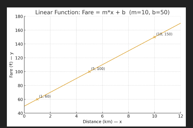
See this graph for a linear function y = mx + b using the taxi example (slope m = 10, intercept b = 50).
What the plot shows:
- The straight line is the function y = 10x + 50.
- X-axis is Distance (km) and Y-axis is Fare (₹).
- The three highlighted points are the example predictions:
- (1, 60) → ₹60 for 1 km
- (5, 100) → ₹100 for 5 km
- (10, 150) → ₹150 for 10 km
- The intercept at x=0x=0x=0 is y=50y=50y=50 (base fare), and the slope 10 means every extra km adds ₹10 to the fare.
Why Linear Functions Important In DS?
- Foundation of Regression Models: Linear regression is one of the most widely used machine learning techniques that is directly based on this concept.
- Easy to Intercept: Linear functions give a clear, human-readable relationship.
- Great for Predictions: You can easily estimate future values using past patterns
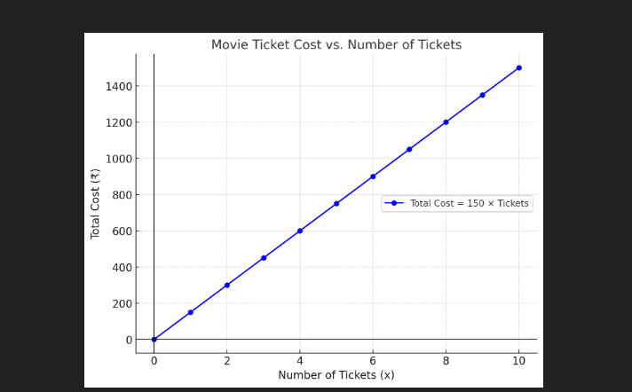
Real-Life Example of Linear Functions
Imagine you are watching the movie in the theatre, and each ticket costs ₹150. If you buy x number of tickets, then your total cost (y) will increase linearly.
y = 150x
Python Code For Creating Graph
import matplotlib.pyplot as plt

# Number of tickets (x-axis)
tickets = [0, 1, 2, 3, 4, 5, 6, 7, 8, 9, 10]

# Total cost (y-axis) -> y = 150 * x
cost = [150 * x for x in tickets]

# Plot the graph
plt.figure(figsize=(7,5))
plt.plot(tickets, cost, marker='o', color='blue', label="y = 150x")

# Labels and title
plt.title("Linear Function Example: Movie Ticket Cost", fontsize=14)
plt.xlabel("Number of Tickets (x)", fontsize=12)
plt.ylabel("Total Cost (y)", fontsize=12)
plt.grid(True, linestyle="--", alpha=0.6)
plt.legend()
plt.show()
Output:
Plotting a Linear Function with Python
Using Python and libraries like Matplotlib, we can visualize a linear function.
import numpy as np
import matplotlib.pyplot as plt

# Let's imagine a simple rule: y grows as 3 times x, plus a fixed start of 5.
def rule_of_growth(x):
    slope = 3         # How fast y increases with each step of x
    start_point = 5   # Where the line begins when x = 0
    return slope * x + start_point

# Create a set of x values from -8 to 8
x_line = np.linspace(-8, 8, 50)   # 50 evenly spaced points
y_line = rule_of_growth(x_line)

# Now, let's draw the line
plt.figure(figsize=(7,5))  # make the plot a bit larger
plt.plot(x_line, y_line, color="darkgreen", linewidth=2, label="y = 3x + 5")

# Add extra touches to make graph friendly
plt.scatter(0, rule_of_growth(0), color="red", zorder=5, label="Intercept (x=0)")
plt.axhline(0, color="gray", linestyle="--", linewidth=0.8)  # x-axis
plt.axvline(0, color="gray", linestyle="--", linewidth=0.8)  # y-axis

plt.title("Visualizing a Linear Growth Rule", fontsize=14)
plt.xlabel("Input (x)")
plt.ylabel("Output (y)")
plt.legend()
plt.grid(True)
plt.show()
Understanding Slope and Intercept
1) Slope (m): This represents the “rise over run” or the rate of change.
- Think of slope as the speed or intensity of change.
- If the slope is positive, the line climbs upwards, which means as x grows, y also grows.
- If the slope is negative, the line goes downwards, which means as x grows, y decreases.
2) Y-Intercept (b): The y-intercept represents the starting point of y when x=0. It is a baseline value in the function and provides a reference point for the line on the graph.
- The intercept is the starting point of the line when x = 0.
- It shows: “Even if you have no x, what is the value of y?”
- On a graph, it’s where the line touches the y-axis.
Linear Functions in Data Science Applications
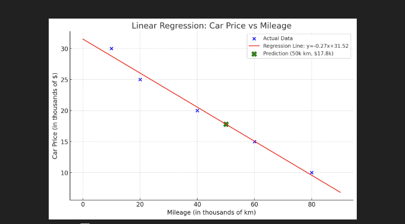
1. Linear Regression
Linear regression aims to find the linear relationship between independent (predictor) and dependent (response) variables by determining the best-fitting line through a dataset.
Example of Linear Regression
Imagine we want to predict the price of a car based on its mileage
import numpy as np
from sklearn.linear_model import LinearRegression

# Mileage of cars (in thousands of km)
mileage = np.array([10, 20, 40, 60, 80]).reshape(-1, 1)

# Corresponding car prices (in thousands of dollars)
price = np.array([30, 25, 20, 15, 10])

# Build linear regression model
model = LinearRegression()
model.fit(mileage, price)

# Extract slope and intercept
slope = model.coef_[0]
intercept = model.intercept_

print("Slope (m):", slope)
print("Intercept (b):", intercept)

# Predict price of a car with 50,000 km mileage
predicted = model.predict([[50]])
print("Predicted Price for 50k mileage:", predicted[0])
Output:
2. Feature Scaling and Normalization
Linear functions are also used in normalization techniques. Machine learning models get confused if one feature is in millions, like salary, and another in tens, like age. For this problem, we use linear scaling that compresses values into a smaller range.
For example:
import numpy as np

# Raw feature values (salary in dollars)
salary = np.array([25000, 50000, 75000, 100000, 125000])

# Apply manual min-max normalization
scaled_salary = (salary - salary.min()) / (salary.max() - salary.min())

print("Original:", salary)
print("Scaled:", scaled_salary)
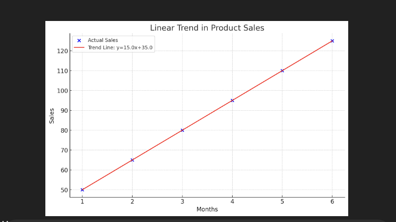
3. Trend Analysis
Linear functions also help us capture straight-line trends in data over time.
Example: Suppose we track monthly sales of a new product:
import numpy as np
import matplotlib.pyplot as plt

# Months (1 to 6)
months = np.array([1, 2, 3, 4, 5, 6])

# Sales (in units)
sales = np.array([50, 65, 80, 95, 110, 125])

# Fit a linear trend line
m, b = np.polyfit(months, sales, 1)  # slope and intercept

# Predicted sales for trend line
trend_line = m * months + b

plt.scatter(months, sales, color="blue", label="Actual Sales")
plt.plot(months, trend_line, color="red", label=f"Trend Line: y={m:.1f}x+{b:.1f}")
plt.xlabel("Months")
plt.ylabel("Sales")
plt.title("Linear Trend in Product Sales")
plt.legend()
plt.grid(True)
plt.show()
Output of this code:
Linear Functions in Multiple Regression
In a simple linear function, we only have one input (x) to predict an output (y). But in the real world, outcomes are rarely influenced by just one factor.
Example: The price of a house doesn’t depend only on its size. It may also depend on:
- The size of the house (in sq. ft.)
- Number of bedrooms
- Location score (how good the area is)
So, instead of one slope, we now have multiple slopes, one for each predictor.
The formula looks like this: y=m1x1+m2x2+m3x3+…+b
- y = output (predicted value, like price)
- x1,x2,x3… = input features
- m1,m2,m3… = slopes (effect of each feature)
- b = intercept (baseline value when all x’s = 0)
Example of Multiple Linear Regression in Python
import numpy as np
from sklearn.linear_model import LinearRegression

# Sample data: predictors are size and number of bedrooms, response is price
X = np.array([[500, 1], [800, 2], [1200, 3], [1500, 4], [1800, 4]])
y = np.array([150, 200, 300, 350, 400])

# Create and fit the model
model = LinearRegression()
model.fit(X, y)

# Display coefficients (slopes) and intercept
print("Coefficients:", model.coef_)
print("Intercept:", model.intercept_)
Advantages and Limitations of Linear Functions
Advantages:
- Simple and Interpretable: Linear functions are easy to understand and interpret, making them useful for simple predictive models.
- Efficient to Compute: Linear functions don’t need heavy mathematical power or expensive machines. Even with millions of data points, they can be trained and used quickly because the calculations are straightforward.
Limitations:
- Limited Flexibility: Linear functions draw a straight line, but real-world data isn’t always straight.
- Sensitive to Outliers: Extreme values can distort the linear relationship, impacting model accuracy.
Exercise For Students
Imagine you run a small coffee shop. You collected data for 7 days: how many people visited your shop and how much total money you earned from coffee sales.
Here’s your dataset:
| Visitors (x) | Coffee Sales in ₹ (y) |
|---|---|
| 20 | 400 |
| 35 | 700 |
| 50 | 1000 |
| 65 | 1300 |
| 80 | 1600 |
| 100 | 2000 |
| 120 | 2400 |
Questions for Students
- Write the linear function that best describes the relationship between visitors (
x) and sales (y).- Hint: Look at how sales increase when visitors increase.
- Interpret the slope of the function.
- What does the slope tell you about sales per visitor?
- Predict the sales if:
- 150 people visit in a day.
- 10 people visit in a day.
- Discussion:
- If one day, a company books a party order of ₹5000 with only 10 visitors, will the linear function still work? Why or why not?
Learn More About Data Science
- What is data in data science?
- What is a database table in data science?
- How to use Python in data science?
- Python DataFrame in data science?
- What are the functions in data science?

M.Sc. (Information Technology). I explain AI, AGI, Programming and future technologies in simple language. Founder of BoxOfLearn.com.