How Data Preparation Works In Data Science?

We learned some definitions about data preparation in previous topics, but now we will learn in depth how Data Preparation actually works in data science.

When you first collect data, it usually doesn’t come in a perfect format. For example:

• We collect student exam records from different schools.
• Some schools use “M” and “F” for gender, others write “Male” and “Female”.
• Some students might have a missing score in one subject, and some entries are unnecessary.

If we try to analyze or build a machine learning model directly on this hardest data, the result will be wrong or misleading.

Data preparation is a crucial step in data science that transforms raw data into a clean, usable format for analysis and modelling.

Why Data Preparation is Important

The raw data contains inconsistencies, errors, or irrelevant information, which can generate an inaccurate analysis or unreliable model predictions. So we ensure the following rules:

1. Data Quality is Improved: Remove errors and inconsistencies.
2. Insights are Reliable: Clean data leads to more accurate analysis and insights.
3. Models Perform Better: Properly prepared data enables machine learning models to learn effectively and produce better results.
4. Efficiency is increased: Clean, well-organized data speeds up the analysis and modelling processes.

Steps in Data Preparation

1. Data Collection
2. Data Cleaning
3. Data Transformation
4. Data Reduction
5. Feature Engineering

Step-by-Step Guide to Data Preparation

1. Data Collection

Data is collected from different sources and multiple formats, like structured tables in a database, semi-structured JSON files, or unstructured text documents. For example, a data scientist may use the Python library pandas to load data from a CSV file:

import pandas as pd

# Load data from a CSV file
df = pd.read_csv('data.csv')

2. Data Cleaning

Data cleaning is the process of identifying and correcting incomplete or irrelevant data. It includes some common tasks like:

• Removing duplicates values
• Handling missing values
• Correcting data types

For example: Handling missing values and duplicates

# Remove duplicates
df = df.drop_duplicates()

# Fill missing values with the mean
df.fillna(df.mean(), inplace=True)

3. Data Transformation

Transformation means converting data into a good format. This can include changing data types, scaling numerical values, encoding categorical variables or creating new columns.

• Encoding Categorical Variables: Many machine learning algorithms require numerical input, so categorical data needs to be converted to numbers.
• Scaling and Normalization: Scaling adjusts the range of numerical values, which can improve model performance.

For example: Encoding categorical variables and scaling numerical data

from sklearn.preprocessing import LabelEncoder, MinMaxScaler

# Encode a categorical column
label_encoder = LabelEncoder()
df['Category'] = label_encoder.fit_transform(df['Category'])

# Scale numerical columns
scaler = MinMaxScaler()
df[['Age', 'Income']] = scaler.fit_transform(df[['Age', 'Income']])

4. Data Reduction

This method reduces the thousands and millions of rows smartly to maintain the speed and efficiency.

Example: Reducing dimensions using PCA (Principal Component Analysis)

from sklearn.decomposition import PCA

# Reduce dataset to 2 dimensions
pca = PCA(n_components=2)
reduced = pca.fit_transform(df[['Age', 'Salary']])

5. Feature Engineering

Feature engineering involves creating new features from existing data that can improve model performance. This includes the following terms:

• Summarize data in meaningful ways.
• Extracting Date Information, such as the extract year, month or day from date-time columns.
• Construct features based on domain knowledge, like calculating age from a birth date.

Example: Feature engineering with date and age

# Extracting year and month from a date column
df['Year'] = pd.DatetimeIndex(df['Date']).year
df['Month'] = pd.DatetimeIndex(df['Date']).month

# Calculate age from birth year
current_year = 2024
df['Age'] = current_year - df['Birth_Year']

Important Code Example for Data Preparation

Now, we write one that cleans, transforms, and analyses the customer dataset. It means converting raw data into clean, structured data.

import pandas as pd
from sklearn.preprocessing import MinMaxScaler, LabelEncoder

# ------------------------------
# Step 1: Create a sample dataset (instead of reading CSV)
# ------------------------------
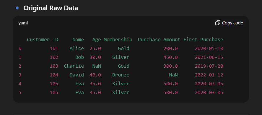
data = {
    'Customer_ID': [101, 102, 103, 104, 105, 105],  # Duplicate ID on purpose
    'Name': ['Alice', 'Bob', 'Charlie', 'David', 'Eva', 'Eva'],
    'Age': [25, 30, None, 40, 35, 35],  # Missing value in Age
    'Membership': ['Gold', 'Silver', 'Gold', 'Bronze', 'Silver', 'Silver'],
    'Purchase_Amount': [200, 450, 300, None, 500, 500],  # Missing value in Purchase
    'First_Purchase': ['2020-05-10', '2021-06-15', '2019-07-20', '2022-01-12', '2020-03-05', '2020-03-05']
}
df = pd.DataFrame(data)

print("🔹 Original Raw Data:")
print(df)

# ------------------------------
# Step 2: Remove Duplicates
# ------------------------------
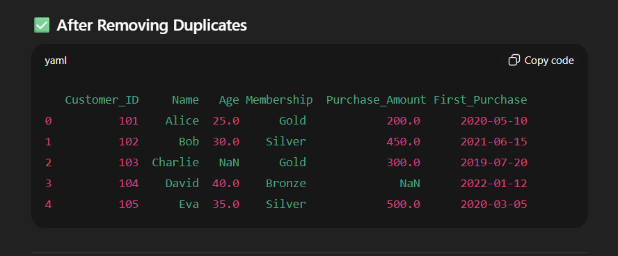
df = df.drop_duplicates(subset=['Customer_ID'])
print("\n After Removing Duplicates:")
print(df)

# ------------------------------
# Step 3: Handle Missing Values
# ------------------------------
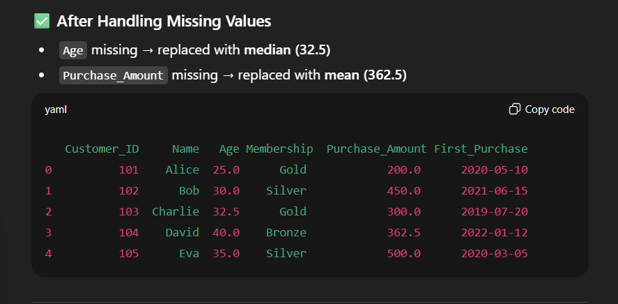
df['Age'].fillna(df['Age'].median(), inplace=True)  # Replace missing Age with median
df['Purchase_Amount'].fillna(df['Purchase_Amount'].mean(), inplace=True)  # Replace missing Purchase with mean

print("\n After Handling Missing Values:")
print(df)

# ------------------------------
# Step 4: Encode Categorical Data
# ------------------------------
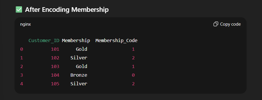
encoder = LabelEncoder()
df['Membership_Code'] = encoder.fit_transform(df['Membership'])

print("\n After Encoding Membership:")
print(df[['Customer_ID', 'Membership', 'Membership_Code']])

# ------------------------------
# Step 5: Feature Engineering
# ------------------------------
df['First_Purchase'] = pd.to_datetime(df['First_Purchase'])
df['Customer_Tenure'] = 2025 - df['First_Purchase'].dt.year  # Years since first purchase

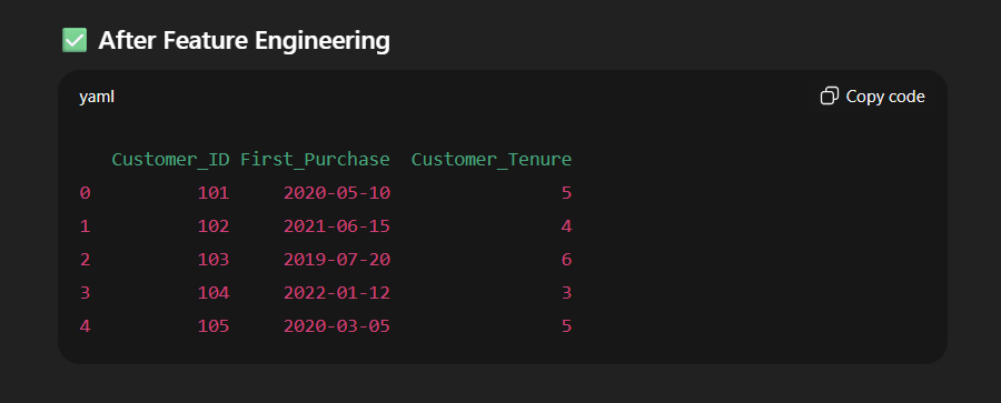
print("\n After Feature Engineering:")
print(df[['Customer_ID', 'First_Purchase', 'Customer_Tenure']])

# ------------------------------
# Step 6: Feature Scaling
# ------------------------------
scaler = MinMaxScaler()
df[['Purchase_Amount', 'Age']] = scaler.fit_transform(df[['Purchase_Amount', 'Age']])

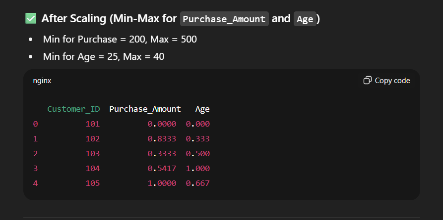
print("\n After Scaling:")
print(df[['Customer_ID', 'Purchase_Amount', 'Age']])

# ------------------------------
# Final Clean Data
# ------------------------------
print("\n Final Prepared Data:")
print(df.head())

• Write this code in your own logic and understand how it’s work.

Output of this code:

Simple Exercise of Data Preparation

“Data Preparation on Retail Store Dataset”

A small retail store maintains customer purchase data in Excel. The data is messy because the shopkeeper manually enters information. Your task is to clean, transform, and prepare the dataset for further analysis.

Given Raw Data (Sample):

Customer_ID	Name	Age	Membership	Purchase_Amount	Join_Date
101	Alice	25	Gold	200	2020-05-10
102	Bob	NaN	Silver	450	2021-06-15
103	Charlie	30	Gold	NaN	2019-07-20
104	David	40	Bronze	300	2022-01-12
105	Eva	35	Silver	500	2020-03-05
105	Eva	35	Silver	500	2020-03-05

Your Tasks:

1. Data Cleaning
   • Remove duplicate customers.
   • Fill in the missing Age with the median age.
   • Fill in the missing Purchase_Amount with the average purchase amount.
2. Data Transformation
   • Encode Membership levels (Bronze, Silver, Gold) into numerical codes.
   • Scale Purchase_Amount into a range of 0–1.
3. Feature Engineering
   • Extract Year and Month from Join_Date.
   • Create a new column Customer_Tenure = 2025 – Join_Year.
4. Final Step
   • Show the final cleaned DataFrame with columns:
     Customer_ID, Name, Age, Membership_Code, Purchase_Amount, Customer_Tenure.

Learn About Data Science

• What is data in data science?
• What is a database table in DS?
• How to use Python in Data Science?
• Data science functions